Getting Started with phyloPal

library(phyloPal)
library(dplyr)
library(ggplot2) 
library(cowplot) 
library(ggplotify)

Overview

phyloPal is designed around a common bottleneck in microbiome data visualization: the gap between having processed abundance data and producing figures that are both publication-ready and honest about compositional structure. The package provides a connected workflow — taxonomy cleaning, data aggregation, color palette generation, and plotting — where each step feeds naturally into the next. Palettes are aware of taxonomic hierarchy, alluvial plots are aware of which taxa are shared versus unique across groups, and combined dendrogram-alluvial figures keep beta diversity and composition aligned in the same panel.

The examples in this vignette use a subset of the GlobalPatterns dataset from the phyloseq package, covering five habitat types: Terrestrial, Oceanic, Freshwater, Brackish, and Freshwater creek.

Installation

phyloPal is available from GitHub. The devtools package is required for installation:

# install.packages("devtools")
devtools::install_github("mwslawinska/phyloPal")

Example data

phyloPal ships with a subset of the GlobalPatterns dataset from the phyloseq package, filtered to five habitat types.

data(example_microbiome)
data(em_metadata)
data(em_otu)

# What does it look like?
glimpse(example_microbiome) # long-format ASV table with RA column
#> Rows: 269,024
#> Columns: 14
#> $ SampleID    <chr> "CL3", "CC1", "SV1", "LMEpi24M", "SLEpi20M", "AQC1cm", "AQ…
#> $ OTU         <chr> "549322", "549322", "549322", "549322", "549322", "549322"…
#> $ Counts      <dbl> 0, 0, 0, 0, 1, 27, 100, 130, 1, 0, 0, 0, 0, 0, 0, 0, 0, 0,…
#> $ Depth       <dbl> 864077, 1135457, 697509, 2117592, 1217312, 1167748, 235718…
#> $ RA          <dbl> 0.000000e+00, 0.000000e+00, 0.000000e+00, 0.000000e+00, 8.…
#> $ SampleType  <fct> Soil, Soil, Soil, Freshwater, Freshwater, Freshwater (cree…
#> $ Habitat     <chr> "Terrestrial", "Terrestrial", "Terrestrial", "Freshwater",…
#> $ Description <fct> "Calhoun South Carolina Pine soil, pH 4.9", "Cedar Creek M…
#> $ Kingdom     <chr> "Archaea", "Archaea", "Archaea", "Archaea", "Archaea", "Ar…
#> $ Phylum      <chr> "Crenarchaeota", "Crenarchaeota", "Crenarchaeota", "Crenar…
#> $ Class       <chr> "Thermoprotei", "Thermoprotei", "Thermoprotei", "Thermopro…
#> $ Order       <chr> NA, NA, NA, NA, NA, NA, NA, NA, NA, NA, NA, NA, NA, NA, NA…
#> $ Family      <chr> NA, NA, NA, NA, NA, NA, NA, NA, NA, NA, NA, NA, NA, NA, NA…
#> $ Genus       <chr> NA, NA, NA, NA, NA, NA, NA, NA, NA, NA, NA, NA, NA, NA, NA…
glimpse(em_metadata) # sample metadata
#> Rows: 14
#> Columns: 4
#> $ SampleID    <fct> CL3, CC1, SV1, LMEpi24M, SLEpi20M, AQC1cm, AQC4cm, AQC7cm,…
#> $ SampleType  <fct> Soil, Soil, Soil, Freshwater, Freshwater, Freshwater (cree…
#> $ Habitat     <chr> "Terrestrial", "Terrestrial", "Terrestrial", "Freshwater",…
#> $ Description <fct> "Calhoun South Carolina Pine soil, pH 4.9", "Cedar Creek M…
glimpse(em_otu)
#>  num [1:19216, 1:14] 0 0 0 0 0 0 7 0 153 3 ...
#>  - attr(*, "dimnames")=List of 2
#>   ..$ : chr [1:19216] "549322" "522457" "951" "244423" ...
#>   ..$ : chr [1:14] "CL3" "CC1" "SV1" "LMEpi24M" ...

Workflows

1. Data preparation and taxonomy cleaning

phyloPal works with long-format ASV/OTU tables where RA is already calculated per ASV/OTU.

A built-in taxonomy cleaner replace_incertae_sedis_NAs() standardizes hierarchical taxonomy columns by normalizing common “Incertae sedis” variants (e.g. “Incertae_Sedis”, “incertae sedis”), filling missing child ranks from stable parent ranks (e.g. a missing Family becomes “Rhizobiales, unclassified” if Order is known), and replacing empty or uninformative entries with "unknown".

All other phyloPal functions call this cleaner internally by default (clean_taxonomy = TRUE), so explicit pre-cleaning is optional but recommended when you want full control over the taxonomy before aggregation.

em_cleaned <- example_microbiome %>%
replace_incertae_sedis_NAs()

glimpse(em_cleaned)
#> Rows: 269,024
#> Columns: 14
#> $ SampleID    <chr> "CL3", "CC1", "SV1", "LMEpi24M", "SLEpi20M", "AQC1cm", "AQ…
#> $ OTU         <chr> "549322", "549322", "549322", "549322", "549322", "549322"…
#> $ Counts      <dbl> 0, 0, 0, 0, 1, 27, 100, 130, 1, 0, 0, 0, 0, 0, 0, 0, 0, 0,…
#> $ Depth       <dbl> 864077, 1135457, 697509, 2117592, 1217312, 1167748, 235718…
#> $ RA          <dbl> 0.000000e+00, 0.000000e+00, 0.000000e+00, 0.000000e+00, 8.…
#> $ SampleType  <fct> Soil, Soil, Soil, Freshwater, Freshwater, Freshwater (cree…
#> $ Habitat     <chr> "Terrestrial", "Terrestrial", "Terrestrial", "Freshwater",…
#> $ Description <fct> "Calhoun South Carolina Pine soil, pH 4.9", "Cedar Creek M…
#> $ Kingdom     <chr> "Archaea", "Archaea", "Archaea", "Archaea", "Archaea", "Ar…
#> $ Phylum      <chr> "Crenarchaeota", "Crenarchaeota", "Crenarchaeota", "Crenar…
#> $ Class       <chr> "Thermoprotei", "Thermoprotei", "Thermoprotei", "Thermopro…
#> $ Order       <chr> "Thermoprotei, unclassified", "Thermoprotei, unclassified"…
#> $ Family      <chr> "unknown", "unknown", "unknown", "unknown", "unknown", "un…
#> $ Genus       <chr> "unknown", "unknown", "unknown", "unknown", "unknown", "un…

2. Data aggregation and color palettes

Before plotting barplots, raw ASV-level data must be aggregated to the desired taxonomic level. process_barplot_data() handles aggregation, normalization, and low-abundance grouping in one step.

Low-abundance handling

A key decision is how to handle low-abundance taxa — those below low_abundance_threshold. The keep_ratype argument controls this: - "collapse" (simpler): all taxa below the threshold are relabelled as “low abundant” and merged into a single bin. This keeps the plot clean and is the right choice when you only care about the dominant taxa. - "separate" (more flexible): low-abundance taxa are flagged but their original identity is preserved in a <tax_level>_original column. The plot-level label becomes "low abundant", but the true taxon name is retained for downstream use.

The low_abundance_basis argument controls when the threshold is applied: - "per_sample": taxa are flagged as low abundant within each individual sample before aggregation. - "post_aggregation": the threshold is applied after averaging across samples or groups.

Aggregation function

The agg_fun argument controls how relative abundances are combined when multiple ASVs map to the same taxon within a sample: - "sum" adds them together, giving the total relative abundance of that taxon in the sample. - "mean" instead averages across ASVs, which is rarely wanted at the within-sample level but can make sense in specific workflows. In most cases, use agg_fun = "sum".

Sample-level aggregation

em_barplot_processed <- process_barplot_data(
  em_cleaned,
  tax_level = "Class",
  group_vars = c("SampleType", "SampleID", "Habitat"),
  low_abundance_basis = "per_sample",
  low_abundance_threshold = 0.01,
  agg_fun = "sum",
  keep_ratype = "separate",
  clean_taxonomy = FALSE
)


em_barplot_processed2 <- process_barplot_data(
  example_microbiome,
tax_level = "Class",
group_vars = c("SampleType", "SampleID", "Habitat"),
low_abundance_threshold = 0.01,
keep_ratype = "collapse",
clean_taxonomy = TRUE,
preserve_higher_taxonomy = T
)

glimpse(em_barplot_processed)
#> Rows: 1,467
#> Columns: 6
#> $ SampleType     <fct> Freshwater, Freshwater, Freshwater, Freshwater, Freshwa…
#> $ SampleID       <chr> "LMEpi24M", "LMEpi24M", "LMEpi24M", "LMEpi24M", "LMEpi2…
#> $ Habitat        <chr> "Freshwater", "Freshwater", "Freshwater", "Freshwater",…
#> $ Class          <chr> "Actinobacteria", "Alphaproteobacteria", "Betaproteobac…
#> $ Class_original <chr> "Actinobacteria", "Alphaproteobacteria", "Betaproteobac…
#> $ RA             <dbl> 2.099578e-01, 2.797942e-02, 9.945164e-02, 5.051917e-02,…
glimpse(em_barplot_processed2)
#> Rows: 188
#> Columns: 6
#> $ SampleType <fct> Freshwater, Freshwater, Freshwater, Freshwater, Freshwater,…
#> $ SampleID   <chr> "LMEpi24M", "LMEpi24M", "LMEpi24M", "LMEpi24M", "LMEpi24M",…
#> $ Habitat    <chr> "Freshwater", "Freshwater", "Freshwater", "Freshwater", "Fr…
#> $ Phylum     <chr> "Actinobacteria", "Bacteroidetes", "Bacteroidetes", "Cyanob…
#> $ Class      <chr> "Actinobacteria", "Flavobacteria", "Sphingobacteria", "Nost…
#> $ RA         <dbl> 2.099578e-01, 5.051917e-02, 4.535482e-02, 4.927715e-01, 2.3…

Group-level aggregation and barplot

Rather than keeping individual samples, data can be aggregated to the group level — for example, averaging relative abundances across all samples of the same SampleType. This is useful when you have many samples per group and want a single representative bar per group, or when you want to compare broad habitat-level patterns rather than sample-level variation. To do this, pass the grouping variables to group_vars and set normalize_by to the same variables — this tells process_barplot_data() to normalize within groups rather than within individual samples. The resulting data frame has one row per taxon per group, ready for plotting with plot_taxonomic_barplot().

em_processed_grouped2 <- process_barplot_data(
  example_microbiome,
  tax_level = "Class",
  group_vars = c("SampleType", "Habitat"),
  normalize_by = c("SampleType", "Habitat"),
  low_abundance_threshold = 0.01,
  preserve_higher_taxonomy = TRUE,
  low_abundance_basis = "per_sample",
  agg_fun = "sum",
  keep_ratype = "separate"
)

Color palettes

generate_palette_hcl() generates perceptually uniform HCL palettes for any number of taxa. HCL (Hue-Chroma-Luminance) colors are preferred for scientific visualization because equal steps in HCL space correspond to equal perceived differences in color — unlike RGB-based palettes where some colors appear much brighter or more saturated than others.

barplot_pal <- generate_palette_hcl(
  data = em_barplot_processed,
  tax_level = "Class",
  fixed_colors_enabled = TRUE,
  fixed_colors_position = "end",
  palette_list = c("Reds", "Purples", "BrwnYl", "Blues", "TealGrn"),
  cmax = 65,
  luminance = c(20,90),
    power = 1.2,
    shuffle = FALSE)

Grouped palette for sample metadata

generate_grouped_palette() assigns colors from the same color family to items sharing a higher-level group — for example, all freshwater sample types in green tones, all oceanic sample types in blue tones. Beyond facet strip coloring, this palette is useful whenever consistent color coding across multiple figure types is needed: if barplot facet strips, dendrogram labels, and beta-diversity ordination plots are colored by the same habitat palette, all figures in a panel share a common visual language and the reader only needs to learn the color scheme once. This is particularly valuable when plotting multiple samples per group — for example, PCoA or NMDS plots where individual samples are colored by their higher-level group membership.


habitat_palette <- generate_grouped_palette(
  data = em_cleaned,
  group_col = "Habitat",
  item_col = "SampleType",
  palette_map = list(
    "Terrestrial" = "BrwnYl",
    "Oceanic" = "Blues",
    "Freshwater" = "Greens",
    "Brackish" = "PuRd"
  ),
  luminance = 65,
  power = 1.2
)

Grouped palette for taxa

The principle used in generate_grouped_palette() can be applied to taxonomic palettes, too. When datasets contain many taxa, a flat palette where colors are assigned arbitrarily can make it hard to orient visually. generate_palette_hcl() supports optional hierarchical grouping via group_by_higher_tax and group_palette_map — all families belonging to Proteobacteria get blue tones, all Actinobacteria get red tones, and so on. This makes the biological structure of the community visible at a glance rather than requiring careful legend inspection. However, hierarchical grouping is recommended only for smaller datasets with fewer than ~10 higher-level taxa — synthetic communities are a typical use case. For complex natural communities with many phyla or classes, the ungrouped palette is typically more interpretable, as too many color families become difficult to distinguish.

em_processed_grouped <- process_barplot_data(
  example_microbiome,
  tax_level = "Class",
  group_vars = c("SampleType", "Habitat"),
  normalize_by = c("SampleType", "Habitat"),
  low_abundance_threshold = 0.1,
  preserve_higher_taxonomy = TRUE,
  low_abundance_basis = "per_sample",
  agg_fun = "sum",
  keep_ratype = "separate"
)

barplot_pal_grouped <- generate_palette_hcl(
  data = em_processed_grouped,
  tax_level = "Class",
   group_by_higher_tax = "Phylum",
   order_by_higher_tax = TRUE,
   group_palette_map = list(
     "Actinobacteria" = "Blues",
     "Proteobacteria" = "Greens",
     "Cyanobacteria" = list(palette = "Purple-Orange", side = "right"),
     "Acidobacteria" = list(palette = "Purple-Orange", side = "right"),
     "Bacteroidetes" = "Burg",
     "Verrucomicrobia" = "BrwnYl"),
  fixed_colors_enabled = TRUE,
  fixed_colors_position = "end",
  order_groups = "alphabetical",
  order_within_groups = "alphabetical",
  cmax = 65,
  luminance = c(20,90),
    power = 1.2,
    shuffle = FALSE)

3. Taxonomic barplots

Facet strips — the label bars above or beside each panel in a faceted plot — are a missed opportunity in most microbiome figures. By default they carry only a text label, but coloring them to match a higher-level grouping variable adds a second layer of information without cluttering the plot. For example, if samples are faceted by SampleType but the Habitat each sample type belongs to should also be visible, coloring the strips by habitat lets the reader group panels visually — all freshwater panels share one color, all oceanic panels another — without adding an extra legend or annotation layer.

In base ggplot2 and even with ggh4x, achieving this requires verbose boilerplate code that is easy to get wrong and hard to keep consistent across figures. In phyloPal, you pass a named color vector directly to facet_strip_colors in plot_taxonomic_barplot() — the same vector produced by generate_grouped_palette() — and the coloring is handled automatically. This makes it straightforward to keep strip colors consistent with other plot elements such as dendrogram labels, ordination point colors, or sample metadata annotations across all figures in a panel.

p_barplot <- plot_taxonomic_barplot(
  data = em_barplot_processed,
  tax_level = "Class",
  palette = barplot_pal,
  x_axis_var = "SampleID",
  facet_by = "SampleType",
  facet_strip_colors = habitat_palette,
  theme_obj = theme_phylopal()
) + 
  ggplot2::guides(
    fill = guide_legend(
      ncol = 1
    )
  ) 

p_barplot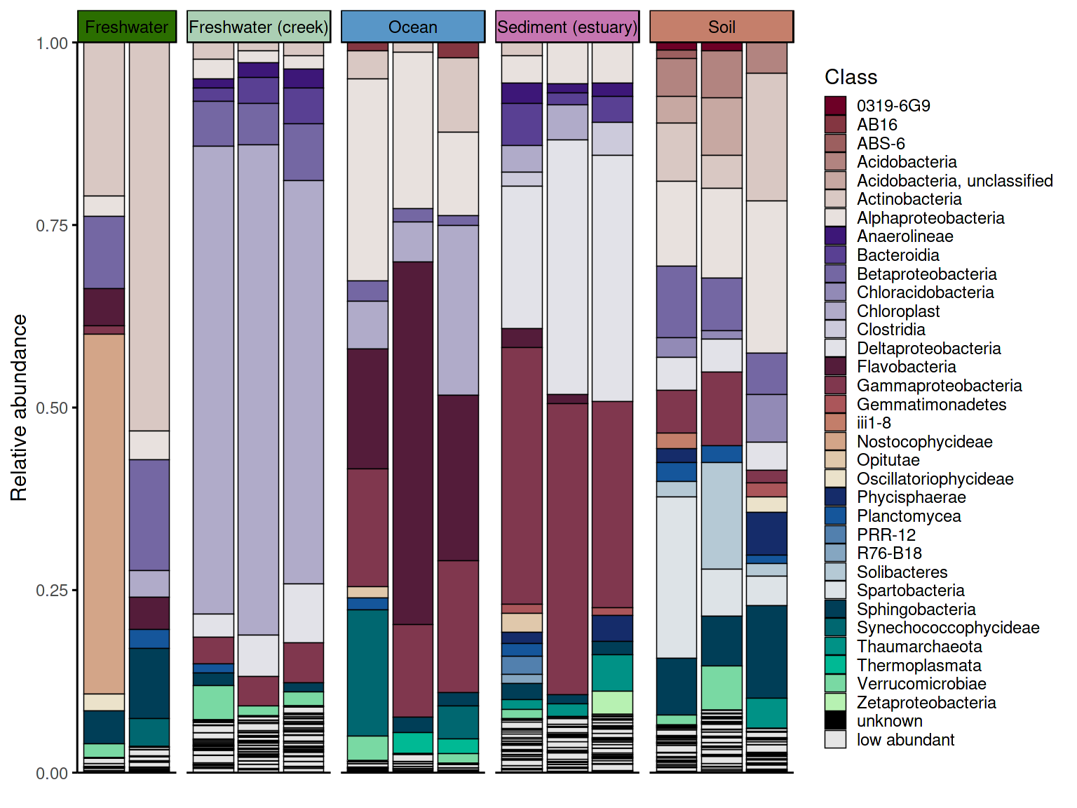

The two data processing approaches produce visually different results. With keep_ratype = "separate", each low-abundance taxon retains its own identity in the <tax_level>_original column and is shown individually in the plot. With keep_ratype = "collapse", all low-abundance taxa are merged into a single "low abundant" bin, producing a cleaner barplot. The choice depends on whether the identity of rare taxa matters for interpretation.

p_barplot2 <- plot_taxonomic_barplot(
  data = em_barplot_processed2,
  tax_level = "Class",
  palette = barplot_pal,
  x_axis_var = "SampleID",
  facet_by = "SampleType",
  facet_strip_colors = habitat_palette,
  theme_obj = theme_phylopal()
) + 
  ggplot2::guides(
    fill = guide_legend(
      ncol = 1
    )
  ) 

p_barplot2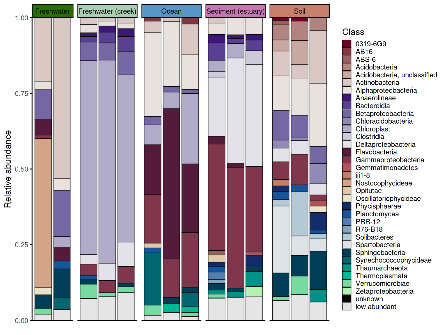

Group-level barplot

Using the group-level aggregated data prepared in the previous section, plot_taxonomic_barplot() produces one bar per group rather than one bar per sample — useful for comparing broad habitat-level patterns across conditions.

p_barplot_grouped2 <- plot_taxonomic_barplot(
  data = em_processed_grouped2,
  tax_level = "Class",
  palette = barplot_pal,
  x_axis_var = "SampleType",
  facet_by = "Habitat",
  theme_obj = theme_phylopal() 
) + 
  ggplot2::guides(
    fill = guide_legend(
      ncol = 1
    )
  )  + theme(axis.text.x = element_text(size =11, angle = 45, hjust = 1, vjust = 1),
    axis.ticks.x = ggplot2::element_line(color = "black", linewidth = 0.4))

p_barplot_grouped2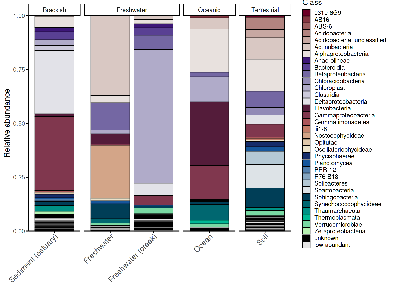

Barplot with hierarchical taxonomic palette

The same group-level data can be plotted with a hierarchically grouped palette, where taxa belonging to the same phylum share a color family. This makes it easier to identify the dominant phylum in each habitat at a glance, without tracing every taxon back to the legend.

p_barplot_grouped <- plot_taxonomic_barplot(
  data = em_processed_grouped,
  tax_level = "Class",
  palette = barplot_pal_grouped,
  x_axis_var = "SampleType",
  facet_by = "Habitat",
  theme_obj = theme_phylopal() 
) + 
  ggplot2::guides(
    fill = guide_legend(
      ncol = 1
    )
  )  + theme(axis.text.x = element_text(size =11, angle = 45, hjust = 1, vjust = 1),
    axis.ticks.x = ggplot2::element_line(color = "black", linewidth = 0.4))

p_barplot_grouped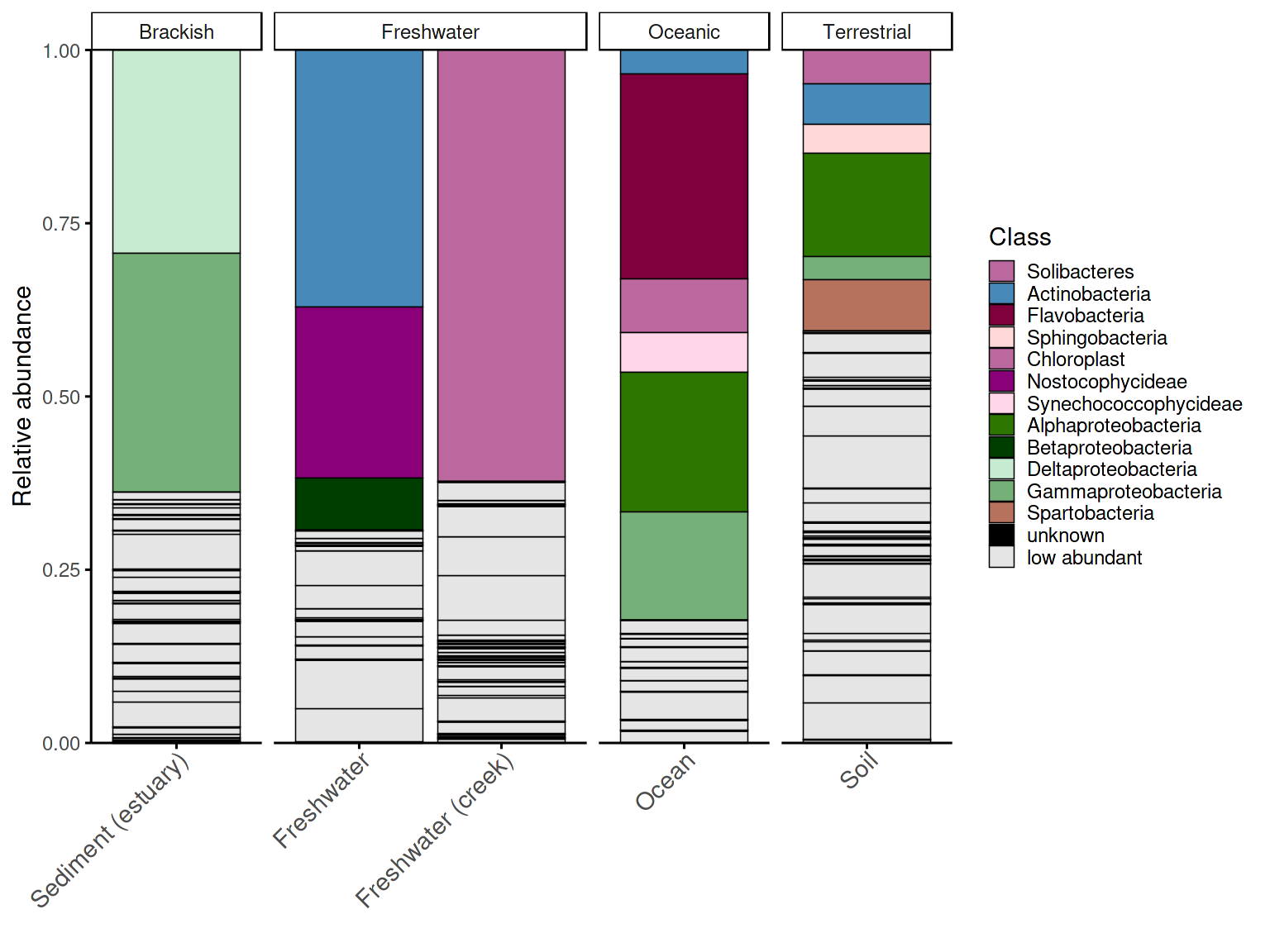

4. Alluvial plots

Alluvial plots (also called Sankey diagrams) show how compositional structure changes across groups — which taxa are present in all groups, which are unique to one, and which shift in abundance between conditions.

Taxa classification

Before plotting, taxa must be classified by their abundance pattern across groups using classify_taxa_patterns(), which assigns each taxon to one of four categories: - shared abundant: present and abundant in all groups - shared low abundant: present in all groups but always below the threshold - unique abundant: abundant in some groups but absent in others - unique low abundant: present in only some groups and always rare

Taxa that are abundant in some groups but low in others are optionally detected as shared mixed abundance (enabled by default). These categories determine both the palette key assigned to each taxon and its stacking position in the plot — shared taxa appear at the bottom, unique taxa toward the top, and fixed categories like "unknown" and "low abundant" always occupy consistent positions.

Step-by-step workflow

The full workflow requires four steps: prepare_alluvial_data() → classify_taxa_patterns() → generate_alluvial_palette() → plot_alluvial(). Each step can be customised independently — for example, using a hierarchical grouped palette, passing special taxa that should never be collapsed into the low-abundance bin, or adjusting classification thresholds independently of the palette.

# arrange the SampleType like you want
example_microbiome$SampleType <- factor(example_microbiome$SampleType, 
levels = unique(example_microbiome$SampleType))

# prepare alluvial data
em_allu <- prepare_alluvial_data(example_microbiome,
tax_level = "Class",
group_col = c("SampleType"),
clean_taxonomy = TRUE
)

# classify taxa patterns according to their abundance
em_allu_classified <- classify_taxa_patterns(
  data = em_allu,
  tax_level = "Class",
  group_col = c("SampleType")
)

glimpse(em_allu_classified)
#> Rows: 885
#> Columns: 7
#> $ SampleType <fct> Soil, Soil, Soil, Soil, Soil, Soil, Soil, Soil, Soil, Soil,…
#> $ Class      <chr> "0319-6G9", "09D2Y74", "12-24", "4C0d-2", "5B-18", "A712011…
#> $ RA         <dbl> 7.304586e-03, 0.000000e+00, 0.000000e+00, 1.013804e-03, 6.0…
#> $ tax_val    <chr> "0319-6G9", "09D2Y74", "12-24", "4C0d-2", "5B-18", "A712011…
#> $ tax_type   <chr> "shared low abundant", "unique low abundant", "unique low a…
#> $ category   <chr> "shared low abundant", "unique low abundant", "unique low a…
#> $ tax_color  <chr> "shared low abundant", "unique low abundant", "unique low a…

# generate palette for the alluvial plot
allu_pal <- generate_alluvial_palette(
    data = em_allu_classified,
  palette_list = c("Reds", "Purples", "BrwnYl", "Blues", "TealGrn"),
  cmax = 65,
  luminance = c(20,90),
    power = 1.2,
    )

# plot the alluvial plot
p_allu <- plot_alluvial(em_allu_classified, 
custom_palette = allu_pal,
tax_level = "Class", 
group_col = "SampleType",
theme_obj = theme_phylopal(),
line_width = 0.2,
x_axis_label = "Sample Type"
) +
ggplot2::theme(axis.text.x = element_text(angle = 45, hjust = 1)) +
  ggplot2::guides(
    fill = guide_legend(
      ncol = 1
    )
  )

p_allu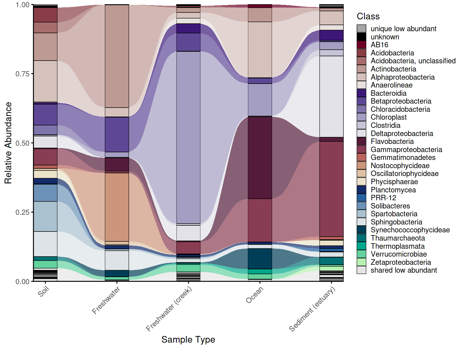

Convenience wrapper

For standard use cases, create_alluvial_plot() wraps the entire workflow into a single call, accepting nested argument lists (prepare_args, classify_args, palette_args, plot_args) passed through to each step. This makes it straightforward to go from raw data to a finished plot in a few lines, while retaining the option to drop into the step-by-step workflow whenever more control is needed.

em_allu_wrapper <- create_alluvial_plot(
  data = example_microbiome,
  tax_level = "Class",
  group_col = "SampleType",
  prepare_args = list(clean_taxonomy = TRUE),
  palette_list = c("Reds", "Purples", "BrwnYl", "Blues", "TealGrn"),
  palette_args = list(
    cmax = 65,
    luminance = c(20, 90),
    power = 1.2
  ),
  plot_args = list(
    theme_obj = theme_phylopal(),
    line_width = 0.2,
    x_axis_label = "Sample Type"
  )
) +
  ggplot2::theme(axis.text.x = ggplot2::element_text(angle = 45, hjust = 1, vjust = 1)) +
  ggplot2::guides(fill = ggplot2::guide_legend(ncol = 1))

em_allu_wrapper

### 5. Alluvial plot combined with dendrogram

While an alluvial plot shows taxonomic composition across groups, it carries no information about how similar those groups are to each other overall. A sample dendrogram addresses this — it clusters groups by beta diversity (here Bray-Curtis dissimilarity) and reveals which communities are most similar in overall structure. Combining both plots in a single figure lets the reader interpret compositional patterns in the context of community-level relationships: groups that cluster closely in the dendrogram are expected to share more taxa in the alluvial plot, and deviations from this expectation become immediately visible.

Building the dendrogram

To create a dendrogram from grouped data (one column per SampleType rather than per sample), first average the ASV/OTU matrix within groups using create_grouped_matrix(), then build the dendrogram with build_dendrogram() and plot it with plot_dendrogram(). The color_by and shape_by arguments in plot_dendrogram() allow metadata variables to be encoded directly on the dendrogram labels, keeping it visually consistent with the alluvial plot and other figures in the panel.

Beta-diversity distances are computed using the vegan package (Oksanen et al., 2022).

em_otu_grouped <- create_grouped_matrix(
asv_matrix = em_otu,
metadata = em_metadata,
sample_col = "SampleID",
group_col= "SampleType",
group_order = "metadata"
)

em_dendrogram <- build_dendrogram(
  mat = em_otu_grouped,
  distance_method = "bray",
  cluster_method = "ward.D2"
)
#> Registered S3 method overwritten by 'dendextend':
#>   method     from 
#>   rev.hclust vegan

em_dendrogram_plot <- plot_dendrogram(
  dend = em_dendrogram,
  metadata = em_metadata,
  label_from = "SampleType",      
  color_by = "SampleType",
  color_palette = habitat_palette,
  point_size = 2,
  orientation = "top",
  shape_by = "Habitat",
  theme_obj = theme_void() + theme(text = element_text(size = 7, color = "black"),
  legend.title = element_text(size = 7, color = "black"),)
)

em_dendrogram_plot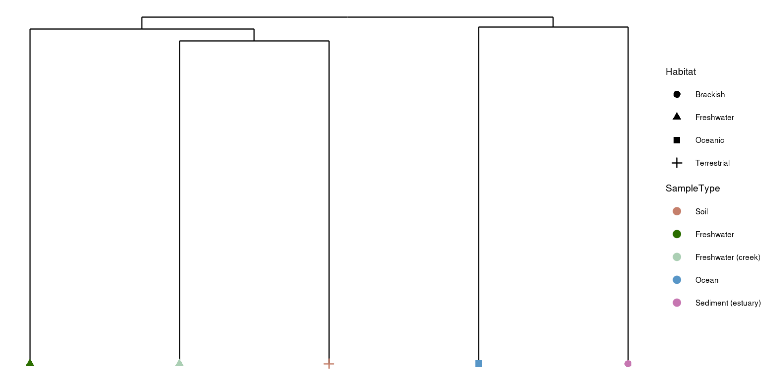

Combining the plots

combine_dendrogram_alluvial() stacks the two plots vertically and aligns their x-axes to the dendrogram leaf order, so the columns of the alluvial plot follow the same left-to-right arrangement as the dendrogram tips. This alignment is handled automatically via leaf_order — without it, the two plots would use independent orderings and the visual connection between them would be lost.

Fine-tuning alignment

A practical challenge when combining dendrograms with alluvial plots is that dendrogram tips rarely fall exactly at integer x positions — branches have varying widths and the outermost tips tend to drift, creating a misalignment between the dendrogram leaves and the alluvial columns beneath them. dend_limits_left and dend_limits_right control the x-axis limits of the dendrogram panel via coord_cartesian(), allowing precise alignment without dropping any data. Increasing dend_limits_left adds space on the left side of the dendrogram panel, pushing the leftmost tip further left — away from the first alluvial column. Increasing dend_limits_right reduces space on the right side, pushing the rightmost tip leftward — toward the center and away from the last alluvial column. The two parameters therefore behave asymmetrically: dend_limits_left pulls the left tip outward, while dend_limits_right pulls the right tip inward. The correct values depend on the number of groups and the specific clustering, so some manual adjustment is expected and normal. For vertical dendrograms, use dend_limits_top and dend_limits_bottom instead.

Legend control

The legend argument controls whether legends are included in the combined figure: "separate" places legends outside the plot area, "omit" removes them entirely, and "together" merges them into one. Omitting legends is useful when full manual control over placement is needed — for example, when using cowplot or ggpubr to arrange legends alongside other figure panels.


p_allu4dend <- create_alluvial_plot(
  data = example_microbiome,
  tax_level = "Class",
  group_col = "SampleType",
  prepare_args = list(clean_taxonomy = TRUE),
  palette_list = c("Reds", "Purples", "BrwnYl", "Blues", "TealGrn"),
  palette_args = list(
    cmax = 65,
    luminance = c(20, 90),
    power = 1.2
  ),
  plot_args = list(
    theme_obj = theme_phylopal(),
    line_width = 0.2,
    x_axis_label = "Sample Type"
  )
) +
  ggplot2::theme(axis.text.x = ggplot2::element_text(angle = 45, hjust = 1)) +
  ggplot2::guides(fill = ggplot2::guide_legend(ncol = 1))


# dendrogram and alluvial with legends
dendrogram_alluplot <- combine_dendrogram_alluvial(
  alluvial_plot   = p_allu4dend +
  scale_y_continuous(expand = c(0,0), breaks = seq(0,1,0.1), limits = c(0,1))+
  ggplot2::guides(fill = guide_legend(ncol =1, title = "Class")),
  dendrogram_plot = em_dendrogram_plot +
  ggplot2::guides(color = guide_legend(ncol = 2, title = "Sample Type"), shape = guide_legend(ncol = 2)),
  dend_position   = "top",
  dend_height     = 0.15,
  strip_alluvial_x = FALSE,
  legend          = "separate",
  legend_source   = "both",       
  legend_position = "right",
  legend_rel_width = 0.75,            
  alluvial_margins    = ggplot2::margin(0, 0, 0, 0, unit = "cm"),
  dendrogram_margins    = ggplot2::margin(0, 0, 0.15, 0, unit = "cm"),
  outer_margins    = ggplot2::margin(0.2, 0.2, 0.2, 0.2, unit = "cm"),
  align = "panel",
  x_expand_zero = TRUE,
  align_x_centers = TRUE,
  leaf_order = em_dendrogram$order,
  overwrite_x_scales = TRUE,
  dend_limits_left = 0.4,  
  dend_limits_right = 0.18
) 
#> Scale for y is already present.
#> Adding another scale for y, which will replace the existing scale.
#> Scale for x is already present.
#> Adding another scale for x, which will replace the existing scale.
#> Scale for x is already present.
#> Adding another scale for x, which will replace the existing scale.
#> Coordinate system already present.
#> ℹ Adding new coordinate system, which will replace the existing one.
grid::grid.draw(dendrogram_alluplot)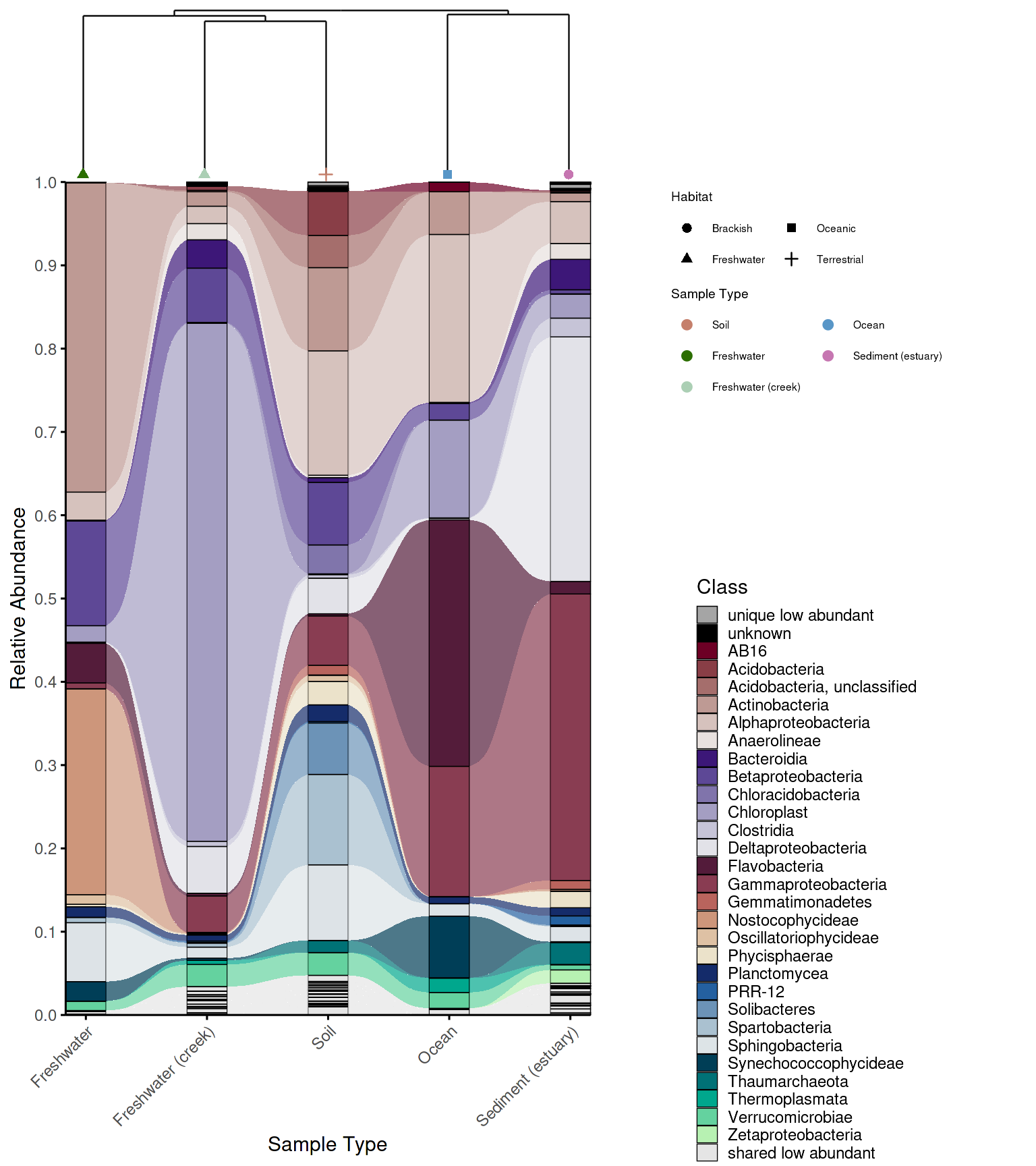

dendrogram_alluplot_control <- combine_dendrogram_alluvial(
  alluvial_plot   = p_allu4dend,
  dendrogram_plot = em_dendrogram_plot,
  dend_position   = "top",
  dend_height     = 0.15,
  strip_alluvial_x = TRUE,
  legend          = "omit",
  legend_source   = "both",       
  legend_position = "right",
  legend_rel_width = 0.75,            
  alluvial_margins    = ggplot2::margin(0, 0, 0, 0, unit = "cm"),
  dendrogram_margins    = ggplot2::margin(0, 0, 0.15, 0, unit = "cm"),
  outer_margins    = ggplot2::margin(0.2, 0.2, 0.2, 0.2, unit = "cm"),
  align = "panel",
  x_expand_zero = TRUE,
  align_x_centers = TRUE,
  leaf_order = em_dendrogram$order,
  overwrite_x_scales = TRUE,
  dend_limits_left = 0.3,  
  dend_limits_right = 0.18
) 
#> Scale for x is already present.
#> Adding another scale for x, which will replace the existing scale.
#> Scale for x is already present.
#> Adding another scale for x, which will replace the existing scale.
#> Coordinate system already present.
#> ℹ Adding new coordinate system, which will replace the existing one.


legend_alluplot <- ggpubr::get_legend(p_allu4dend + 
                                            guides(
                                              fill = guide_legend(ncol =1, title = "Class")))


legend_dendrogram <- ggpubr::get_legend(
  em_dendrogram_plot + 
  ggplot2::guides(color = guide_legend(ncol = 1, title = "Sample Type"), shape = guide_legend(ncol = 1))+
    ggplot2::theme(legend.position = "right", 
          legend.box = "vertical",
          legend.title.position = "top",
          plot.margin = margin(0,0,0,0))
)

p_allu_full <- cowplot::plot_grid(
  cowplot::plot_grid(
    ggplotify::as.ggplot(dendrogram_alluplot_control),
    cowplot::plot_grid(
      legend_dendrogram,
      legend_alluplot,
      rel_heights = c(0.6, 1),
      rel_widths = c(1, 1),
      ncol = 1,
      align = "hv", axis = "tblr"
    ),
    rel_widths = c(1,0.6),
    ncol = 2,
    align = "hv", axis = "tblr"
  )
)

grid::grid.draw(p_allu_full)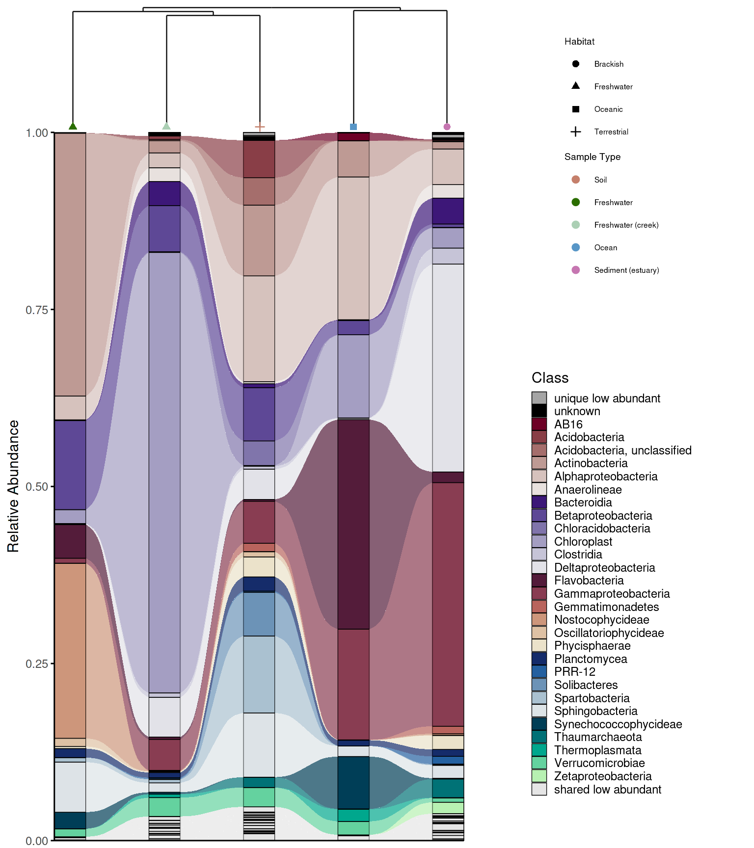

Convenience wrapper

The whole process can be simplified using the create_alluvial_dendrogram_plot() wrapper, which runs the full pipeline — grouping the ASV/OTU matrix, building the dendrogram, preparing and classifying alluvial data, generating the palette, and combining the plots — in a single call.

It takes as input the raw ASV/OTU matrix (asv_matrix, samples as columns and ASVs/OTUs as rows), a metadata data frame, and the long-format ASV/OTU table with pre-calculated RA (alluvial_data).

Arguments for each internal step are passed as named lists: build_dendrogram_args and plot_dendrogram_args control the dendrogram, while alluvial_args accepts nested prepare_args, classify_args, palette_args, and plot_args forwarded to the respective alluvial functions. Layout parameters like dend_limits_left, dend_limits_right, and legend_rel_width are direct arguments rather than nested, since they are commonly adjusted.

The function returns a named list containing all intermediate objects — grouped_matrix, dendrogram, dendrogram_plot, alluvial, and combined_plot — so any component can be accessed for further customization or export without rerunning the pipeline.

Use the wrapper for standard workflows and drop into the step-by-step approach when you need to modify an intermediate result.

res <- create_alluvial_dendrogram_plot(
  asv_matrix = em_otu,
  metadata = em_metadata,
  sample_col = "SampleID",
  group_col  = "SampleType",
  alluvial_data = example_microbiome,
  tax_level = "Class",
  dend_color_palette = habitat_palette,
  dend_shape_by = "Habitat",
  theme_alluvial = theme_phylopal(),
  theme_dendrogram = ggplot2::theme_void(),
  alluvial_args = list(
    return_all = TRUE,
    prepare_args = list(clean_taxonomy = TRUE),
    classify_args = list(low_abundance_threshold = 0.01),
    palette_args = list(
      palette_list = c("Reds", "Purples", "BrwnYl", "Blues", "TealGrn"),
      cmax = 65,
      luminance = c(20, 90),
      power = 1.2
    ),
    plot_args = list(
      line_width = 0.2,
      x_axis_label = "Sample Type"
    )
  ),
  post_plot_guides   = list(      # guides applied to alluvial
    fill = ggplot2::guide_legend(ncol = 1, title = "Class")
  ),    
  dend_limits_left = 0.4,  
  dend_limits_right = 0.18, 
  combine_args = list(
    legend_rel_width = 0.5,
    strip_alluvial_x = TRUE,  
    alluvial_margins = ggplot2::margin(0, 0, 0, 0, unit = "cm"),
    outer_margins    = ggplot2::margin(0.2, 0.5, 0.2, 0.2, unit = "cm") 
  )
)
#> Scale for x is already present.
#> Adding another scale for x, which will replace the existing scale.
#> Coordinate system already present.
#> ℹ Adding new coordinate system, which will replace the existing one.

p_em_alluvial_dend_wrapper <- res$combined_plot

grid::grid.draw(p_em_alluvial_dend_wrapper)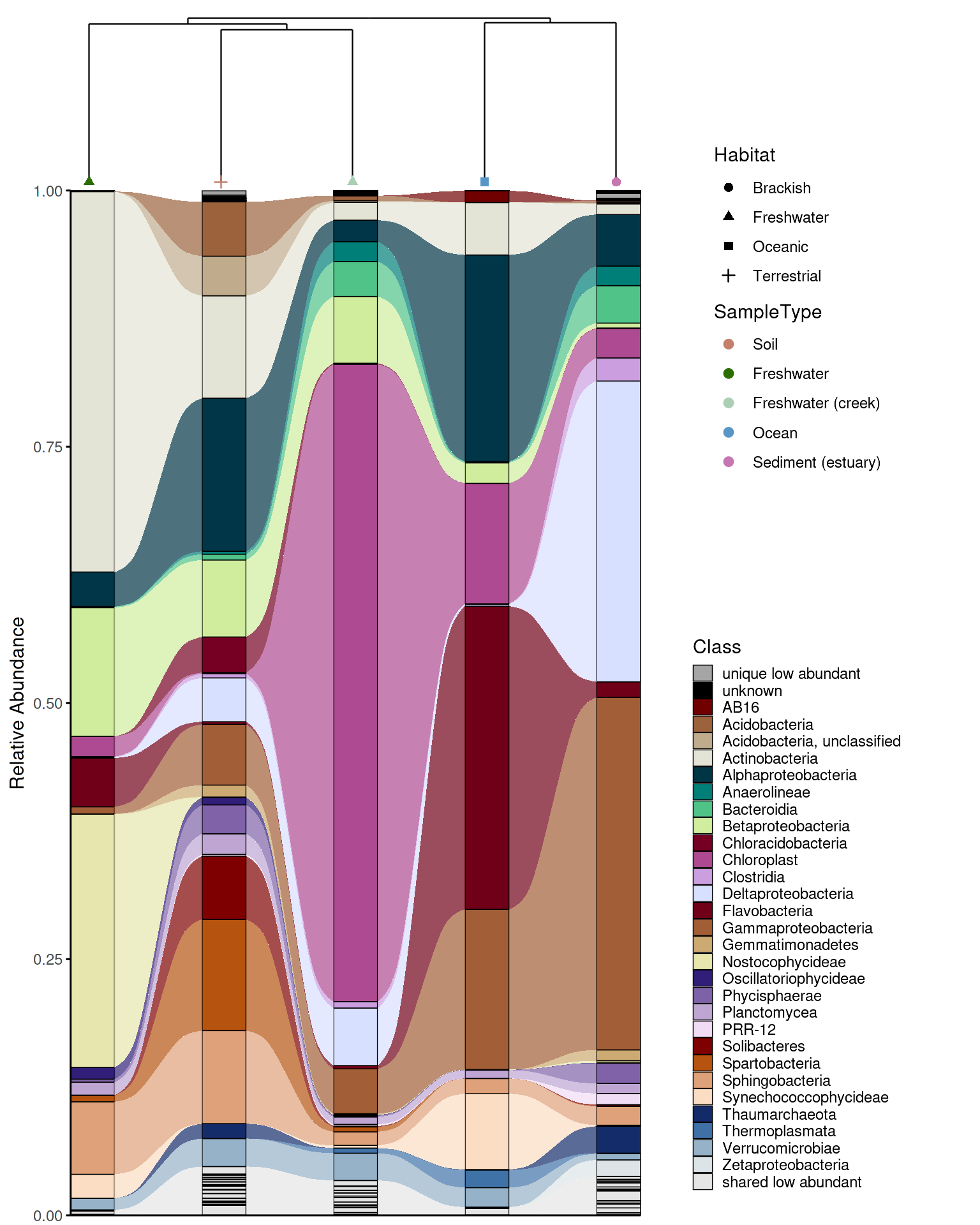

Function reference

Function	What it does
`replace_incertae_sedis_NAs()`	Clean taxonomy: normalize Incertae Sedis, propagate parent taxa
`process_barplot_data()`	Aggregate ASV-level RA to taxonomic level, mark low-abundance taxa
`prepare_alluvial_data()`	Aggregate and complete zeros for alluvial input
`classify_taxa_patterns()`	Classify taxa as shared/unique/mixed-abundance across groups
`generate_palette_hcl()`	HCL palette with optional hierarchical grouping by higher taxonomy
`generate_grouped_palette()`	Assign color families to groups (e.g. for facet strip colors)
`generate_alluvial_palette()`	Alluvial-aware palette respecting shared/unique structure
`add_alpha()`	Add transparency to hex colors
`plot_taxonomic_barplot()`	Stacked barplot with optional colored facet strips
`plot_alluvial()`	Alluvial/Sankey plot
`build_dendrogram()`	Compute Bray-Curtis dendrogram from ASV/OTU matrix
`plot_dendrogram()`	Plot dendrogram with metadata-colored labels
`combine_dendrogram_alluvial()`	Combine alluvial + dendrogram with aligned axes
`create_alluvial_plot()`	Full alluvial workflow wrapper
`create_alluvial_dendrogram_plot()`	Full alluvial + dendrogram wrapper
`theme_phylopal()`	Clean built-in ggplot2 theme

References

Caporaso, J.G., et al. (2011). Global patterns of 16S rRNA diversity at a depth of millions of sequences per sample. PNAS, 108, 4516–4522.

Oksanen, J., et al. (2022). vegan: Community Ecology Package. R package version 2.6-4. https://CRAN.R-project.org/package=vegan

Brunson, J.C. (2020). ggalluvial: Layered Grammar for Alluvial Plots. Journal of Open Source Software, 5(49), 2017.

Citation

If you use phyloPal in your research, please cite: Slawinska MW (2025). phyloPal: Taxonomic Color Palettes and Alluvial-Dendrogram Visualization for Microbiome Data. R package version 0.1.0. https://github.com/mwslawinska/phyloPal

Overview

Installation

Example data

Workflows

1. Data preparation and taxonomy cleaning

2. Data aggregation and color palettes

Low-abundance handling

Aggregation function

Sample-level aggregation

Group-level aggregation and barplot

Color palettes

Grouped palette for sample metadata

Grouped palette for taxa

3. Taxonomic barplots

Colored facet strips

Group-level barplot

Barplot with hierarchical taxonomic palette

4. Alluvial plots

Taxa classification

Step-by-step workflow

Convenience wrapper

Building the dendrogram

Combining the plots

Fine-tuning alignment

Legend control

Convenience wrapper

Function reference

References

Citation

License